Predicting Congestion at Intersections

Driving is a means of travelling that is preferred by many people. We all want to drive efficiently and reach our destination with as little time stuck in a traffic jam as possible. The ability to predict traffic at intersections enables us to plan our course ahead of time and avoid busy streets and intersections. In this project, we attempt to train machine learning models to predict the time it takes to cross an intersection and how congested it is at an intersection.

Data Analysis

Our dataset is retrieved from the Kaggle competition: BigQuery-Geotab Intersection Congestion

Overview of the Dataset

Statistics

Number of features: 13

Feature	~	~	~	~	~
Row ID	Intersection ID	Latitude	Longitude	Entry Street Name	Exit Street Name
Entry Heading	Exit Heading	Hour	IsWeekend	Month	Path¹
Total Time Stopped²: 20%	Total Time Stopped: 40%	Total Time Stopped: 50%	Total Time Stopped: 60%	Total Time Stopped: 80%
Time from First Stop³: 20%	Time from First Stop: 40%	Time from First Stop: 50%	Time from First Stop: 60%	Time from First Stop: 80%
Distance to First Stop⁴: 20%	Distance to First Stop: 40%	Distance to First Stop: 50%	Distance to First Stop: 60%	Distance to First Stop: 80%
City

Number of Records: 857409

Number of unique intersections: 1991

Features of concern

City: Atlanta, Boston, Chicago, Philadelphia
Weekend: if a particular day is a weekend
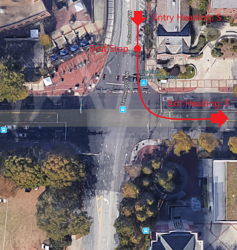
Entry Heading: one of “E”, “NE”, “N”, “NW”, “W”, “SW”, “S”, “SE”
Exit Heading: one of “E”, “NE”, “N”, “NW”, “W”, “SW”, “S”, “SE”

Target Output

Total time stopped at an intersection, 20^th, 50^th, 80^th percentiles
Distance between the intersection and the first place the vehicle stopped and started waiting, 20^th, 50^th, 80^th percentiles

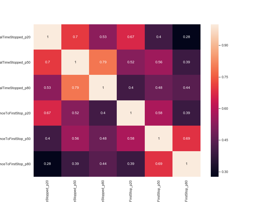
Correlation

Visualizing the data

Example

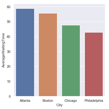
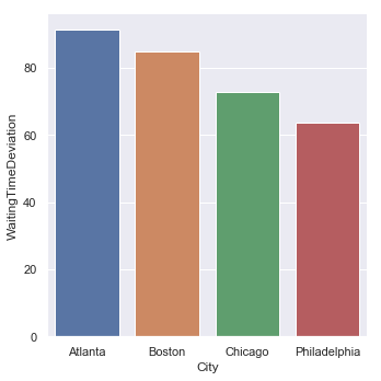
North Avenue and Techwood Drive intersection

Average Waiting Time by City

Average Waiting Time	Standard Deviation

Average First Stopping Distance from the Intersection by City

Average First Stop Distance	Standard Deviation

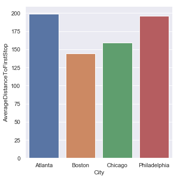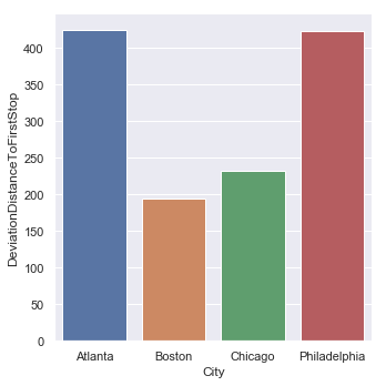Average Time to pass the Intersection since First Stop by City

Average Time from First Stop	Standard Deviation

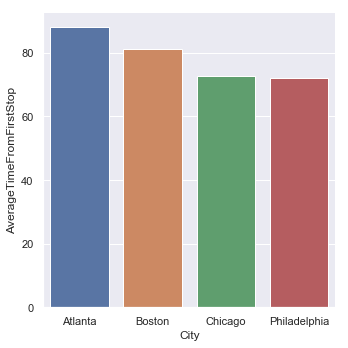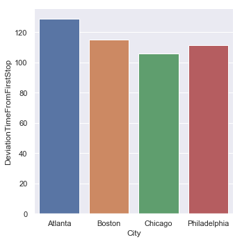Wait time by day: weekdays and weekends

Weekdays	Weekends

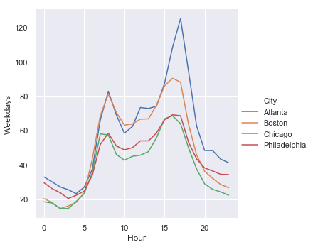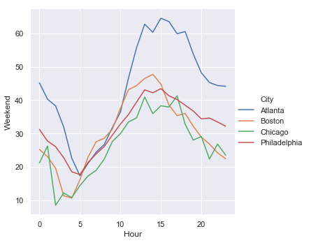By Street

Entry Streets	Exit Street

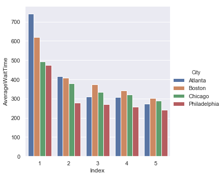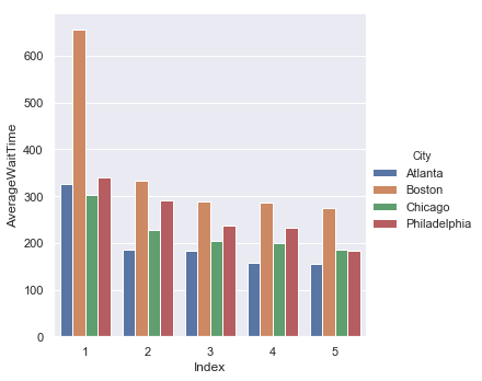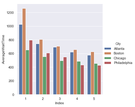
Most Travelled Path

Heat Map of Waiting Times

Our Approach

Note: We changed target outputs from the 6 mentioned above to 2: Total Time Stopped and Distance to First Stop.

Feature Engineering

Turning Directions
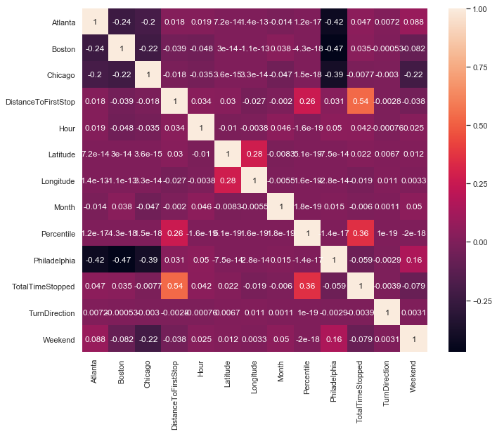
The cardinal directions can be expressed using the following equation: 𝜃/𝜋 where 𝜃 is the angle between the we want to encode direction and the north direction measured clockwise. Ex: 'N' = 0, 'E' = 0.5, 'W' = 1.5

Turning directions = ExitDirection - EntryDirection
Latitudes & Longitudes
We observe that each city has a clear downtown area, so we created a standard scalar for each city in order to encode the distance to the downtown area.
Cities
Since there are 4 cities in the dataset, we used one-hot encoding to transform the “city” feature.
Percentiles

We expect that the percentiles we need to predict are dependent on each other. We created this feature to capture this dependency.
TotalTimeStopped (Output)

The total time stopped at an intersection.
DistanceToFirstStop (Output)
The distance between the intersection and the first place a vehicle stopped while waiting.

Correlation

Machine Learning Models

Regression Models

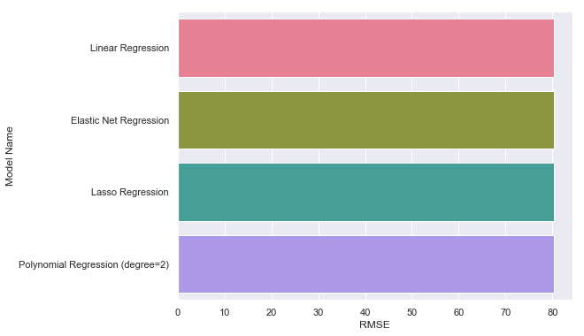
First we tried linear regression, then we applied regularization techniques, including lasso regression and elastic net regression. We also experimented with polynomial regression for degree of 2. After tuning the hyperparameter to improve results on the validation dataset, we observed that the performance are still quite similar as shown below.

Performances (RMSE)

Linear Regression: 80.237
Elastic Net Regression: 80.239
Lasso Regression: 80.238
Polynomial Regression (degree 2): 80.238

RMSE of Regressors

Gradient Boost Machines

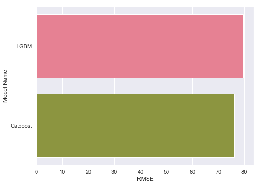
We tried Catboost regressor and LightGBM regressor. For Catboost regressor, we applied techniques such as bagging and L2 regularization. For LightGBM, we transformed the dataset into matrices, and applied techniques such as specifying categorical features to predict the outputs. We see a better performance in LightGBM than Catboost.

Performances (RMSE)

Catboost: 79.628
LGBM: 76.009

RMSE of Gradient Boost Machines

Neural Network

We built a simple neural network that consists of three linear layers, and we used Relu as the activation function. The input size into the neural network is (batch size x 11), and output size is (batch size x 2) [We trained on 11 features, and outputted 2 target values]. The rmse is 78.574, which beats the benchmark (rmse = 80), but is slightly worse than LightGBM.

Performance (RMSE)

Neural Network: 78.574

Random Forest

We applied grid search technique to find the optimal set of parameters such as number of estimators, maximum depth and number of jobs. Our best random forest regression model achieved a high performance of rmse = 75.001, which is the best amongst all models we tried.

Performance (RMSE)

Random Forest: 75.001

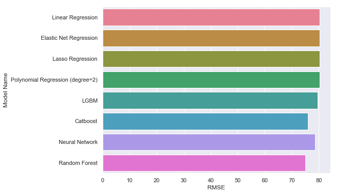
Comparing all Models

RMSE

Discussion

Overall, we used supervised learning, and four categories of models were tested. We observe that all models provided similar results. Among these, random forest, neural network, LightGBM and catboost all beat benchmark (rmse = 80). In addition, random forest regression model has the best performance, achieving top 30% on the leaderboard on Kaggle.

During our training process, we also found that using random split and k-fold (k = 5) gives over optimistic results. So we only used random split to train our models. This gave us more consistent rmse scores when comparing predicted results on validation set and predicted results on test set.

Intersection-Congestion-Prediction

This repository contains content for GA Tech CS-4641 Project for Group 19

References

- Google Big Query. BigQuery-Geotab Intersection Congestion. July 2019. 30 October 2019.
- Kohavi, Ron. “A study of cross-validation and bootstrap for accuracy estimation and model selection.” International Joint Conference on Artificial Intelligence. 1995. 1137-1145
- Kotsiantis, Sotiris B. and I Zaharakis. “Supervised machine learning: A review of classification techniques.” Emerging artificial intelligence applications in computer engineering (2007): 3-24
- Peng, Chao-Ying Joanne, Kuk Lida Lee, and Gary M. Ingersoll. “An introduction to logistic regression analysis and reporting.” The Journal of Educational Research 96.1 (2002): 3-14.